The theory behind the so-called perceptron, basically the key building block of artificial neural networks and thereby all modern deep learning or “AI” models, is almost as old as the transistor. So if these algorithms are as old as computers themselves, why did it take more than half a century before they entered the main stage of science and technology? The answer is: It’s complicated. Literally. Running existing models is relatively easy, but training them is not. Especially not if one has real world applications in mind. But before we can look at some of the breakthroughs that brought us to where we are today, let’s take a step back and understand how artificial neural networks actually work. The first step when recreating the brain in a computer is obviously to look at how the brain does it’s computing. Below is a sketch of a neuron, the basic computing component of virtually every animal’s nervous system.
Diagram of a Neuron | Source: Wikipedia
There are also other cell types found in the brain, but neurons are responsible for the electro-chemical communication processes that can not just transmit but also manipulate information. When activated, a neuron fires an electrical pulse along the axon to all connected neurons. The strength of the eventually received signal is determined by the synaptic connections between individual neurons. When the total incoming signal surpasses an excitation threshold, the receiving neuron will fire as well. In a simplified way, we can break this down into its components by using a graph-like structure of nodes and edges with weights for each connection. In a fully connected network, each neuron in a layer is connected to each neuron in the next layer.
Given a set of numeric input values, we can formally compute the value of the first neuron in the middle layer on the left as the sum over all inputs multiplied by their respective connection’s weight as
If we group all weights for all neurons together in a matrix, we can write the values of the second layer as one vector:
We then apply an activation function f that mimics the process in a neuron where the output is only active when the input reaches a certain threshold. The output of this network for a given input x is then
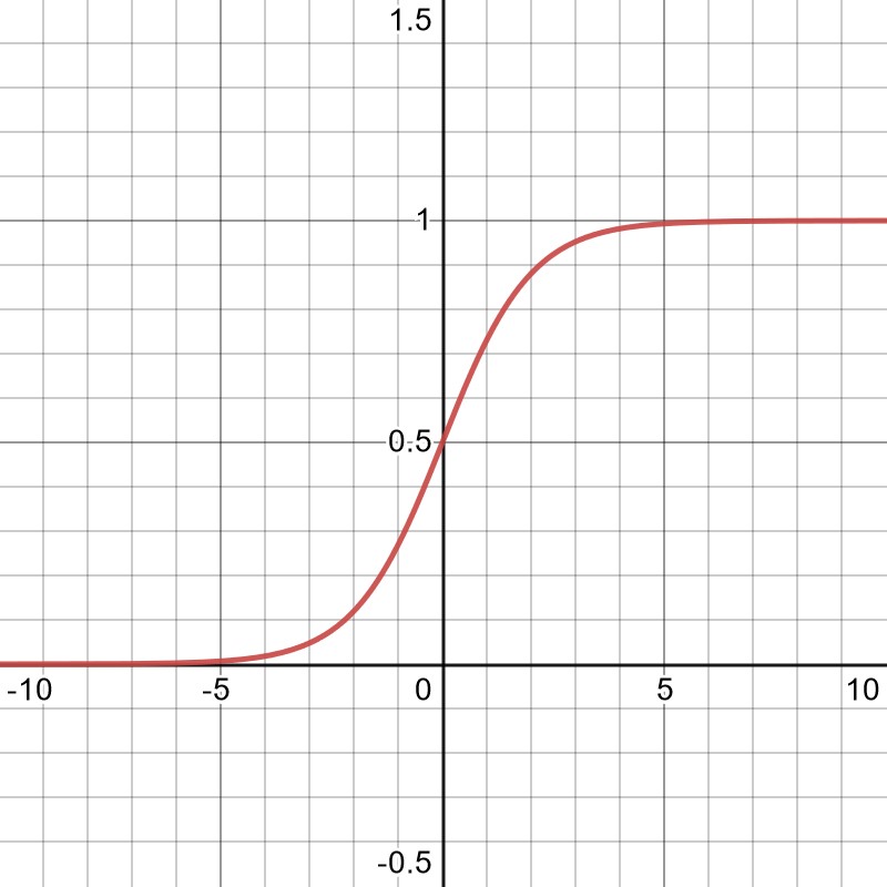
A common choice for the activation function is a so-called sigmoid function,
shown in the plot below. The shape of the function and its continuous behaviour differ from something you would find in biological systems, but it turns out to be sufficient.
Made with desmos.com
By adding an additional bias neuron with a fixed value of one to the input and hidden layers, the activation graph of individual neurons can be shifted left and right, while the weights of the other inputs scale it up and down. Combined with the other neurons, it is easy to create arbitrary-dimensional functions of any continuous shape by tuning the entries encoded in the weights of the two matrices. This simple setup might not sound like much, but the multi layer feedforward architecture is actually capable of approximating any continuous function over compact domains. In principle, this means that any algorithm that takes an input and produces an output could be realized as such a neural network. The big question is: How do we get the weights? For incredibly tiny networks, it may even be possible to tune them by hand, but this becomes infeasible very fast. Instead, the networks are trained on existing, ground truth datasets by matching given inputs to pre-labelled outputs. This way, one can calculate the “error” or difference between the model’s output and the desired output and then use the process of backpropagation to iteratively update the model parameters. Backpropagation makes use of automatic differentiation and gradient descent to slightly lower the error at every step of the iteration. Gradient descent works by looking at the function that generated the error (i.e. the whole computational graph of the model) and taking its partial derivatives with respect to the trainable parameters. By changing the parameters in the direction of their derivative that lowers the total error, the model can iteratively be tuned to produce the desired output. Normally, calculating derivatives of complicated nested functions like the one described above can be very tedious, but if one knows the derivative of the activation function it can be easily automated. Even better, since essentially all computer chips calculate by breaking down functions into simple operations of addition and multiplication, calculating derivatives of these nested functions can be done with a simple application of the chain rule.
Over time it became clear that realistic problems would require extremely large networks. The first problem here lies in the fact that for such large networks, the derivatives of a normal sigmoid-like activation function tend to vanish. This can be easily seen by looking at the graph above and imagining many neurons contributing to the total input that would appear on the x-axis. By going too far left or right on the plot, the function changes very little, making it hard to update the network parameters in a reasonable way. This problem was solved by moving further away from the original, biological inspirations and instead introducing the rectified linear unit, or ReLU as activation function.
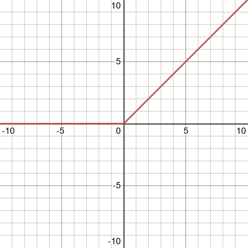
Made with desmos.com
This function is extremely simple – it is just x for x>0 and 0 otherwise. However, it retains just enough nonlinearity to sufficiently capture complex behaviour inside neural networks and it has the added benefit that its gradient doesn’t vanish – at least not for large values of x. It is also much easier to calculate than the complicated nonlinear sigmoid functions, making models a lot more performant. Today there are many variations of ReLU, but it has become a cornerstone of Deep Learning models and is used virtually everywhere, including in the models available in Transkribus.
Another major problem faced by bigger networks is that with an increasing number of parameters, overfitting becomes more prevalent. To ensure that the model does not merely replicate the training data but also learns to generalize from it, regularization methods turned out to be very helpful. One of the most established ones makes use of so-called dropout layers. During training, a dropout layer takes one layer of hidden neurons and sets the output of randomly chosen neurons to zero – regardless of their input. This forces the network to diffuse any information and prevents reliance on certain correlations that might be prevalent in the training data. Dropout layers have become another cornerstone of deep learning and are also used for training models in Transkribus.
Something we haven’t mentioned yet but which is also very important for large models is how to set the parameters initially. After all, the iterative training process has to start somewhere. For small networks, it is usually sufficient to just set the parameters randomly according to some probability distribution. This means however, that consecutive layers will be expecting these distributions and a small parameter change in an early layer can lead to huge changes down the road for models with many hidden layers. In order to train these deep networks, it becomes necessary to standardize the inputs for every layer. This is done using a process called batch normalization. It looks at the output of a specific layer for a batch of different inputs and then rescales the output such that the whole set retains certain statistical properties – usually a mean of zero and a variance of one. First proposed in 2015, this technique is now prevalent in almost all deep neural networks, including the ones that are used by Transkribus.
There have been many, many more improvements in the field of artificial neural networks over the years. Some of them were small, while others were real game changers such as convolutional networks, recurrent networks and, more recently, transformers (stay tuned for more on these in future blog posts). Combined, they eventually made it possible to train gigantic networks that can perform incredible tasks. Together with the rise of incredibly powerful parallel computing chips that were originally designed for video games (but turned out to be perfect for training neural networks as well), we now finally have the means to make use of the big-data revolution.
We use cookies to personalize and improve content and services, deliver relevant advertising, and enhance the security of our users. You can check your cookie settings at any time. You can find more information on the use of cookies and cookie settings in our Privacy policy Cookie settingsRejectAccept
Privacy & Cookies Policy
Privacy Overview
This website uses cookies to improve your experience while you navigate through the website. Out of these cookies, the cookies that are categorized as necessary are stored on your browser as they are essential for the working of basic functionalities of the website. We also use third-party cookies that help us analyze and understand how you use this website. These cookies will be stored in your browser only with your consent. You also have the option to opt-out of these cookies. But opting out of some of these cookies may have an effect on your browsing experience.
Necessary cookies are absolutely essential for the website to function properly. This category only includes cookies that ensures basic functionalities and security features of the website. These cookies do not store any personal information.
Cookie
Description
Duration
viewed_cookie_policy
The cookie is set by the GDPR Cookie Consent plugin and is used to store whether or not user has consented to the use of cookies. It does not store any personal data.
1 hour
PHPSESSID
This cookie is native to PHP applications. The cookie is used to store and identify a users' unique session ID for the purpose of managing user session on the website. The cookie is a session cookies and is deleted when all the browser windows are closed.
Advertisement cookies are used to provide visitors with relevant ads and marketing campaigns. These cookies track visitors across websites and collect information to provide customized ads.
Cookie
Description
Duration
VISITOR_INFO1_LIVE
This cookie is set by Youtube. Used to track the information of the embedded YouTube videos on a website.
5 months
IDE
Used by Google DoubleClick and stores information about how the user uses the website and any other advertisement before visiting the website. This is used to present users with ads that are relevant to them according to the user profile.
Analytical cookies are used to understand how visitors interact with the website. These cookies help provide information on metrics the number of visitors, bounce rate, traffic source, etc.
Cookie
Description
Duration
GPS
This cookie is set by Youtube and registers a unique ID for tracking users based on their geographical location
30 minutes
tk_or
This cookie is set by JetPack plugin on sites using WooCommerce. This is a referral cookie used for analyzing referrer behavior for Jetpack
5 years
tk_r3d
The cookie is installed by JetPack. Used for the internal metrics fo user activities to improve user experience
3 days
tk_lr
This cookie is set by JetPack plugin on sites using WooCommerce. This is a referral cookie used for analyzing referrer behavior for Jetpack
1 year
_ga
This cookie is installed by Google Analytics. The cookie is used to calculate visitor, session, camapign data and keep track of site usage for the site's analytics report. The cookies store information anonymously and assigns a randoly generated number to identify unique visitors.
2 years
_gid
This cookie is installed by Google Analytics. The cookie is used to store information of how visitors use a website and helps in creating an analytics report of how the wbsite is doing. The data collected including the number visitors, the source where they have come from, and the pages viisted in an anonymous form.
1 day
matomo
For statistical analysis, we use “Matomo” on this website. This is an open source tool for web analysis. Matomo does not transmit data to servers outside the control of the READ-COOP. Matomo is deactivated when you visit our website. Only if you actively consent will your usage behaviour be recorded anonymously.
1 year
Hubspot
Hubspot, Inc., 25 First Street, Cambridge, MA 02141 USA
HubSpot is a user database management service provided by HubSpot, Inc. We use HubSpot on this website for our online customer support activities.
Performance cookies are used to understand and analyze the key performance indexes of the website which helps in delivering a better user experience for the visitors.
Cookie
Description
Duration
YSC
This cookies is set by Youtube and is used to track the views of embedded videos.
1 year
_gat
This cookies is installed by Google Universal Analytics to throttle the request rate to limit the colllection of data on high traffic sites.